[I] Preface

In a nutshell

This tutorial is, to some extent, a simplified version of my previous tutorial on chromosome-level scaffolding and annotation of the diploid plant Arabidopsis thaliana (2n=2x=10). In this version, I include a Quality Check (QC) assessment step and employ an approach for identifying syntenic blocks commonly used in comparative genomics. Additionally, I have downsized the dataset to include only the smallest chromosome, Chr4 (ca. 22.2 Mbp), which should reduce the overall time required to complete the analysis. The tutorial is part of the workshop Introduction to Bioinformatics and OMICs Data Analysis, conducted at XTBG from February 10–14, 2025 (workshop leader: Dr Guillem Ylla).

Please note that all data used here was produced by Wang B et al., 2021. Additionally, please be aware that this tutorial does not aim to reproduce all analyses from the aforementioned article in detail.

Learning outcomes

After completing this tutorial, you will be able to:

perform a quality check of the raw sequencing data.
assemble a genome of interest using data produced by second- and third-generation sequencing technologies, including Illumina, Oxford Nanopore Technologies (ONT), and Pacific Biosciences Circular Consensus Sequencing (CCS) reads.
scaffold assembled contigs to the scale of full chromosomes using a reference genome.
scaffold assembled contigs to the scale of full chromosomes using Hi-C data.
identify, annotate and mask transposable elements.
annotate genomes using RNA-Seq and protein homology information.
visualise the results.

Keywords

Bioinformatics, Quality Check, ONT sequencing, HiFi sequencing, Illumina sequencing, Hi-C sequencing, RNA sequencing, genome assembly, genome annotation, Synteny, data visualisation.

[II] Conda & sequencing data

Conda, software, and packages

IMPORTANT! Please refer to the aforementioned tutorial on creating and setting up conda environments, as well as package and software installation. Additionally, you may consider switching to mamba over conda.

Downloading raw sequence data

A subset of the Illumina, ONT, HiFi, and Hi-C reads was privately provided to the workshop participants. The files are now available for download through the Zenodo repository.

Subsampling workflow

To reproduce all the steps for data subsampling while keeping only the reads aligned to Chromosome 4, follow the steps below.

[1] Dataset

First, create directories for Illumina, RNA-Seq, Hi-C, HiFi, and ONT data:

Bash

mkdir Illumina RNAseq HiC HiFi ONT

Then, download the following files:

Illumina folder:

Bash

nohup wget ftp://download.big.ac.cn/gsa/CRA004538/CRR302670/CRR302670_f1.fastq.gz > CRR302670_f1.out 2>&1 &
nohup wget ftp://download.big.ac.cn/gsa/CRA004538/CRR302670/CRR302670_r2.fastq.gz > CRR302670_r2.out 2>&1 &

RNAseq folder:

Bash

nohup wget https://sra-pub-run-odp.s3.amazonaws.com/sra/SRR3581356/SRR3581356 > wget_SRR3581356.out 2>&1 & # root
nohup wget https://sra-pub-run-odp.s3.amazonaws.com/sra/SRR3581693/SRR3581693 > wget_SRR3581693.out 2>&1 & # flower
nohup wget https://sra-pub-run-odp.s3.amazonaws.com/sra/SRR3581681/SRR3581681 > wget_SRR3581681.out 2>&1 & # leaf
nohup wget https://sra-pub-run-odp.s3.amazonaws.com/sra/SRR3581705/SRR3581705 > wget_SRR3581705.out 2>&1 & # internode
nohup wget https://sra-pub-run-odp.s3.amazonaws.com/sra/SRR3581706/SRR3581706 > wget_SRR3581706.out 2>&1 & # seed
nohup wget https://sra-pub-run-odp.s3.amazonaws.com/sra/SRR3581708/SRR3581708 > wget_SRR3581708.out 2>&1 & # silique
nohup wget https://sra-pub-run-odp.s3.amazonaws.com/sra/SRR3581703/SRR3581703 > wget_SRR3581703.out 2>&1 & # pedicel

HiC folder:

Unix

nohup wget ftp://download.big.ac.cn/gsa/CRA004538/CRR302669/CRR302669_f1.fastq.gz > CRR302669_f1.out 2>&1 &
nohup wget ftp://download.big.ac.cn/gsa/CRA004538/CRR302669/CRR302669_r2.fastq.gz > CRR302669_r2.out 2>&1 &

HiFi folder:

Unix

nohup wget ftp://download.big.ac.cn/gsa/CRA004538/CRR302668/CRR302668.fastq.gz > CRR302668.out 2>&1 &

ONT folder:

Unix

nohup wget ftp://download.big.ac.cn/gsa/CRA004538/CRR302667/CRR302667.fastq.gz > CRR302667.out 2>&1 &

[2] Chromosome subsetting

Download the reference genome:

Unix

nohup wget https://download.cncb.ac.cn/gwh/Plants/Arabidopsis_thaliana_AT_GWHBDNP00000000/GWHBDNP00000000.genome.fasta.gz > Arabidopsis_genome.out 2>&1 &

Unzip the compressed file:

Unix

unpigz -k -p 4 GWHBDNP00000000.genome.fasta.gz

Check the headers:

Unix

grep ">" GWHBDNP00000000.genome.fasta > GWHBDNP00000000.genome_Chr_list.txt && cat GWHBDNP00000000.genome_Chr_list.txt

It should look like this:

GWHBDNP00000001

Chromosome 1

Complete=F

Circular=F

OriSeqID=chr1

Len=32659241

GWHBDNP00000002

Chromosome 2

Complete=F

Circular=F

OriSeqID=chr2

Len=22712559

GWHBDNP00000003

Chromosome 3

Complete=F

Circular=F

OriSeqID=chr3

Len=26161332

GWHBDNP00000004

Chromosome 4

Complete=F

Circular=F

OriSeqID=chr4

Len=22250686

GWHBDNP00000005

Chromosome 5

Complete=F

Circular=F

OriSeqID=chr5

Len=30093473

Next, we will retain only the shortest chromosome:

Unix

awk -v chr=4 '
BEGIN {FS="\t"} 
$1 ~ />GWHBDNP/ && $2 == "Chromosome " chr {print; flag=1; next} 
$1 ~ />GWHBDNP/ && $2 != "Chromosome " chr {flag=0} 
flag
' GWHBDNP00000000.genome.fasta > Arabidopsis_GWHBDNP00000000_chr4.fasta

Additionally, let’s index the reference genome:

Unix

minimap2 -d Arabidopsis_GWHBDNP00000000_index.mmi GWHBDNP00000000.genome.fasta

And Chromsome 4 to speed up subsequent alignments:

Unix

hisat2-build Arabidopsis_GWHBDNP00000000_chr4.fasta hisat2_Arabidopsis_GWHBDNP00000000_chr4

[3] Trimming and alignment

Next, we will remove adapter sequences and retain only high-quality reads.

Illumina DNA data

Trimming:

Unix

trim_galore \
--cores 8 \
--paired \
--quality 30 \
--length 100 \
--clip_R1 15 \
--clip_R2 15 \
--three_prime_clip_R1 10 \
--three_prime_clip_R2 10 \
--dont_gzip \
CRR302670_f1.fastq.gz CRR302670_r2.fastq.gz

Alignment (do not forget to specify the path for the -x parameter and create the Temp_samtools folder):

Unix

nohup sh -c 'hisat2 \
-p 44 \
--reorder \
--no-mixed \
--no-discordant \
--no-unal \
--sam-no-qname-trunc \
-x hisat2_Arabidopsis_GWHBDNP00000000_chr4 \
-1 CRR302670_f1_val_1.fq \
-2 CRR302670_r2_val_2.fq \
-S - | \
samtools view -@ 44 -Sb -F 4 - | \
samtools sort -@ 44 -m 10G -T /Temp_samtools -o DNA_Illumina_sorted.bam - && \
samtools fastq -@ 22 \
-1 DNA_Illumina_chr4_R1.fastq \
-2 DNA_Illumina_chr4_R2.fastq \
DNA_Illumina_sorted.bam' &

Subsampling. We will keep only 75% of the reads:

Unix

for suffix in R1 R2; do
  seqtk sample -s 77 "DNA_Illumina_chr4_${suffix}.fastq" 0.75 > "DNA_Illumina_chr4_subset_${suffix}.fastq"
done

Illumina RNA data

Convert the SRA files into FASTQ:

Unix

for srr_id in SRR3581706 SRR3581708 SRR3581693 SRR3581681 SRR3581356 SRR3581705 SRR3581703; do
  fasterq-dump --threads 44 --split-files "$srr_id"
done

Trimming:

Unix

parallel -j 4 "nohup trim_galore -q 20 --cores 4 {}.fastq > {}_trim.log 2>&1 &" \
::: SRR3581706 SRR3581708 SRR3581693 SRR3581681 SRR3581356 SRR3581705 SRR3581703

Alignment (do not forget to specify the path for the -x parameter):

Unix

SAMPLES=(SRR3581706 SRR3581708 SRR3581693 SRR3581681 SRR3581356 SRR3581705 SRR3581703)
for SAMPLE in "${SAMPLES[@]}"; do
  nohup bash -c "
  hisat2 -p 12 --no-unal --sam-no-qname-trunc \
  -x hisat2_Arabidopsis_GWHBDNP00000000_chr4 \
  --rna-strandness F \
  -U '${SAMPLE}_trimmed.fq' \
  -S '${SAMPLE}.sam' && \
  samtools view -@ 12 -Sb -F 4 -q 20 '${SAMPLE}.sam' > '${SAMPLE}.bam' && \
  samtools sort -@ 12 -m 10G -o '${SAMPLE}_RNA_Illumina_chr4_subset.bam' '${SAMPLE}.bam' && \
  samtools fastq -@ 12 '${SAMPLE}_RNA_Illumina_chr4_subset.bam' > '${SAMPLE}_RNA_Illumina_chr4_subset.fastq' && \
  rm -f '${SAMPLE}.sam' '${SAMPLE}.bam'
  " > "${SAMPLE}.log" 2>&1 &
done

Illumina Hi-C data

Trimming:

Unix

trim_galore \
--cores 8 \
--paired \
--quality 30 \
--length 100 \
--clip_R1 15 \
--clip_R2 15 \
--three_prime_clip_R1 10 \
--three_prime_clip_R2 10 \
--dont_gzip \
CRR302669_f1.fastq.gz CRR302669_r2.fastq.gz

Alignment (do not forget to specify the path for the -x parameter and create the Temp_samtools folder):

Unix

nohup sh -c 'hisat2 -p 22 --reorder --no-mixed --no-discordant --no-unal --sam-no-qname-trunc \
--no-spliced-alignment \
-x hisat2_Arabidopsis_GWHBDNP00000000_chr4 \
-1 CRR302669_f1_val_1.fq \
-2 CRR302669_r2_val_2.fq \
-S - | \
samtools view -@ 22 -Sb -F 4 - | \
samtools sort -n -@ 22 -m 10G -T /Temp_samtools -o Hi_C_Illumina_chr4.bam - && \
samtools fastq -@ 22 \
-1 Hi_C_Illumina_chr4_R1.fastq \
-2 Hi_C_Illumina_chr4_R2.fastq \
Hi_C_Illumina_chr4.bam' &

PacBio HiFi data

Trimming:

Unix

cutadapt \
-j 20 \
-a "AATGTACTTCGTTCAGTTACGTATTGCT" \
-a "AGAGTACATGGGAGTTGGTTATGGTAAT" \
--quality-cutoff 30 \
-m 5000 \
-M 30000 \
-o HiFi_trimmed.fastq.gz \
CRR302668.fastq.gz

Alignment (do not forget to create the Temp_samtools :

Unix

minimap2 -ax map-hifi -t 44 Arabidopsis_GWHBDNP00000000_chr4.fasta HiFi_trimmed.fastq.gz | \
samtools view -@ 22 -Sb -F 4 -F 256 -F 2048 -q 50 | \
samtools sort -@ 22 -m 10G -T /Temp_samtools -o HiFi_chr4.bam - && \
samtools fastq -@ 22 HiFi_chr4.bam > HiFi_chr4.fastq

Subsampling. We will keep only 75% of the reads:

Unix

seqtk sample -s 77 HiFi_chr4.fastq 0.75 > HiFi_chr4_subset.fastq

ONT data

Trimming:

Unix

porechop --threads 44 -i CRR302667.fastq.gz -o ONT_trimmed.fastq.gz

Correction. Since aligning with uncorrected ONT reads might not be the best approach, we first correct them using NECAT by creating an arabidopsis_config.txt file, where read_list.txt specifies the path to ONT_trimmed.fastq.gz :

PROJECT=Arabidopsis
ONT_READ_LIST=read_list.txt
GENOME_SIZE=135000000
THREADS=44
MIN_READ_LENGTH=10000
PREP_OUTPUT_COVERAGE=40
OVLP_FAST_OPTIONS=-n 500 -z 20 -b 2000 -e 0.5 -j 0 -u 1 -a 1000
OVLP_SENSITIVE_OPTIONS=-n 500 -z 10 -e 0.5 -j 0 -u 1 -a 1000
CNS_FAST_OPTIONS=-a 2000 -x 4 -y 12 -l 1000 -e 0.5 -p 0.8 -u 0
CNS_SENSITIVE_OPTIONS=-a 2000 -x 4 -y 12 -l 1000 -e 0.5 -p 0.8 -u 0
TRIM_OVLP_OPTIONS=-n 100 -z 10 -b 2000 -e 0.5 -j 1 -u 1 -a 400
ASM_OVLP_OPTIONS=-n 100 -z 10 -b 2000 -e 0.5 -j 1 -u 0 -a 400
NUM_ITER=2
CNS_OUTPUT_COVERAGE=40
CLEANUP=1
USE_GRID=false
GRID_NODE=0
GRID_OPTIONS=
SMALL_MEMORY=0
FSA_OL_FILTER_OPTIONS=
FSA_ASSEMBLE_OPTIONS=
FSA_CTG_BRIDGE_OPTIONS=
POLISH_CONTIGS=true

Unix

necat correct arabidopsis_config.txt

Alignment with corrected reads to the reference genome:

Unix

minimap2 -ax map-ont -t 44 GWHBDNP00000000.genome.fasta cns_final.fasta.gz | \
samtools sort -@ 44 -o full_align.bam

Index the bam file:

Unix

samtools index full_align.bam

Extract reads mapping uniquely to Chromosome 4:

Unix

samtools view -@ 22 -b -q 20 -F 256 -F 2048 full_align.bam "GWHBDNP00000004" -o ONT_chr4.bam

And convert BAM to FASTQ:

Unix

samtools fastq -@ 22 ONT_chr4.bam > ONT_chr4.fastq

[4] Sabsampling for the QC chapter

Illumina DNA data

Let’s keep only 5% of the reads for downstream quality checks:

Unix

seqtk sample -s 11 CRR302670_f1.fastq.gz 0.05 | gzip > DNA_Illumina_QC.fastq.gz

PacBio HiFi data

We retain only 1% of the reads:

Unix

seqtk sample -s 77 CRR302668.fastq.gz 0.01 | gzip > HiFi_QC.fastq.gz

ONT data

Here, we also retain only 1% of the reads:

Unix

seqtk sample -s 77 CRR302667.fastq.gz 0.01 | gzip > ONT_QC.fastq.gz

[III] Genome assembly

Recap

Genome assembly is like rebuilding the Great Wall. The original wall is unique, but it has many identical sections (such as watchtowers and repeating brick patterns) repeated along its length. If you break the wall into tiny pieces (similar to how DNA is fragmented during sequencing), rebuilding it perfectly becomes challenging because repeating structures make it difficult to determine how the pieces fit together. To solve this, we can use different sequencing technologies:

Illumina (short reads): provides highly accurate details of small fragments (like individual bricks). However, it struggles with long repetitive sections (e.g., repeated watchtowers), leaving gaps in the reconstruction.
PacBio HiFi (long reads): captures longer sequences and can bridge many repetitive regions. However, it may still fail to resolve extremely long identical sections (e.g., massive fortress-like structures).
ONT PromethION (ultra-long reads): spans entire sections of the wall, revealing how large repeating structures are connected. Drawback: these reads have more errors and need fixing.

Goal: Rebuild the Great Wall (genome) exactly as it was, with no misplaced bricks.

Solution: use ultra-long reads (ONT) to map how giant repeating sections connect; refine the structure with long reads (HiFi) and short reads (Illumina) to fix errors and ensure every brick is in the right place (Figure 1).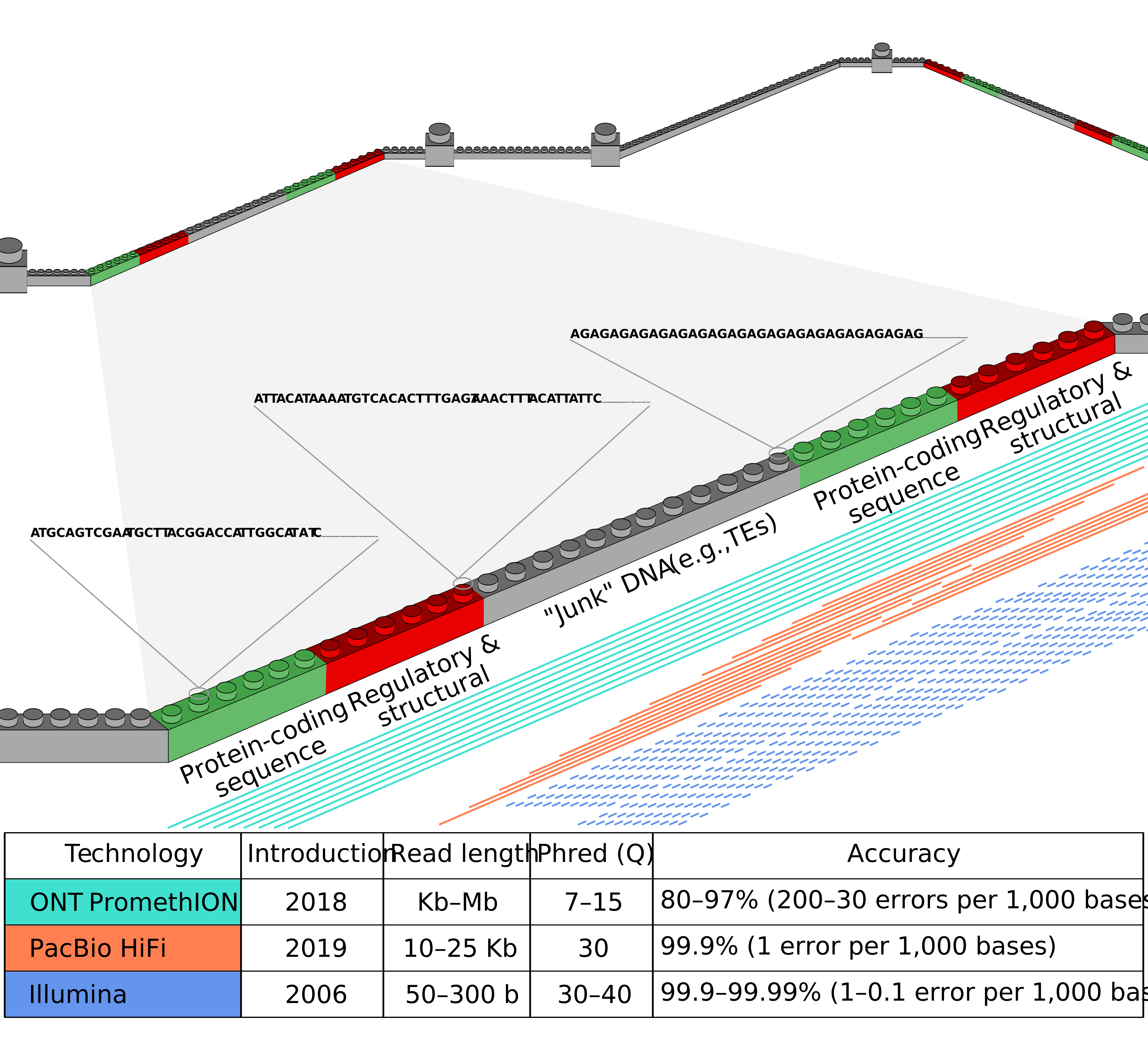

Figure 1. Overview of the sequencing technologies used in this tutorial.

Here, we will use a hybrid genome assembly pipeline, as illustrated in Figure 2.

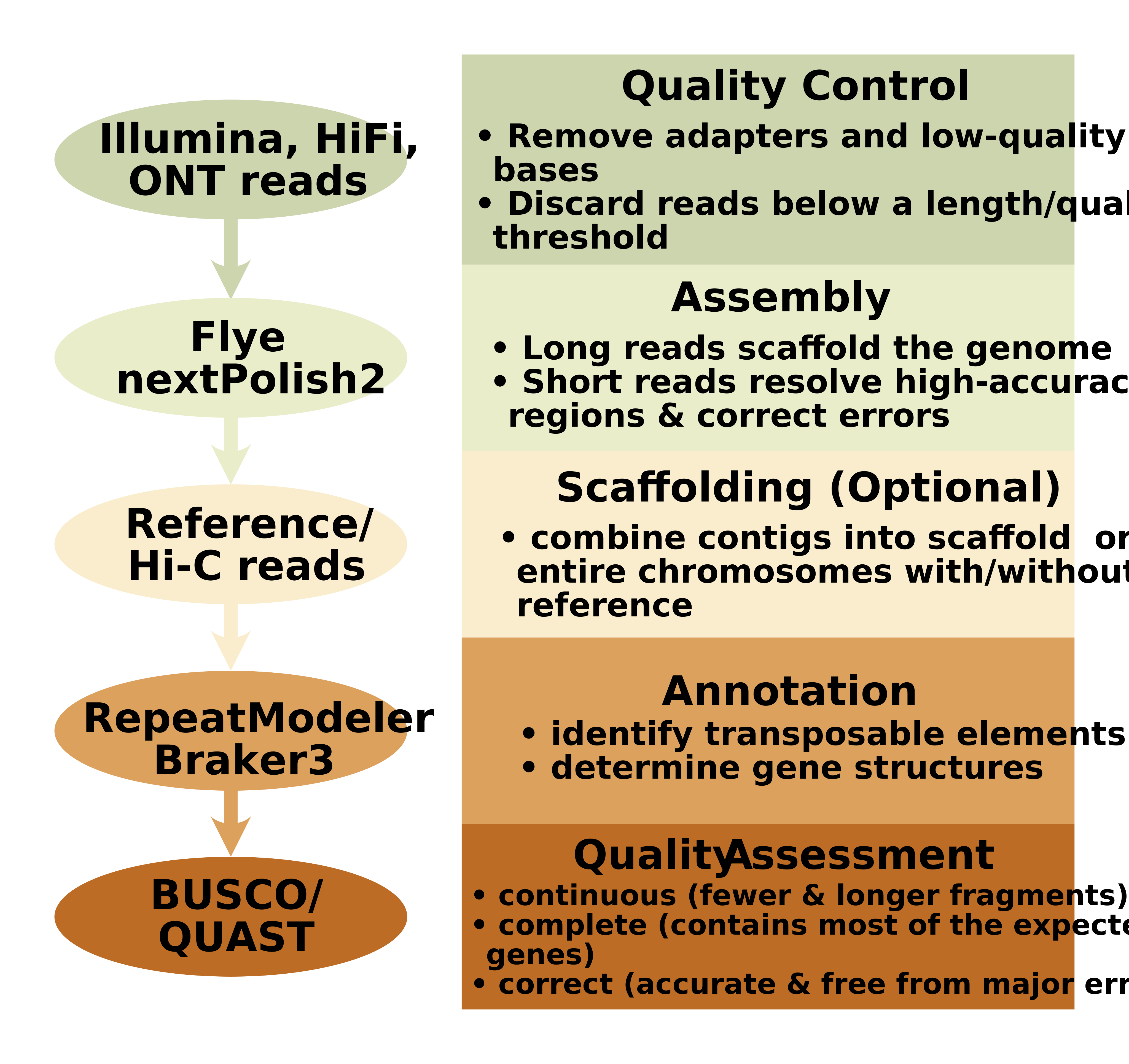
Figure 2. Key steps in the hybrid genome assembly pipeline.

Quality check

Short-Read Sequencing

Let’s perform a quick quality check using Illumina DNA reads:

Unix

fastqc DNA_Illumina_QC.fastq.gz

And check the resulted file DNA_Illumina_QC_fastqc.html (Figure 3):

Figure 3. The FastQC output report.

Now, we will remove adapters (if present), set a quality threshold of 35, retain only sequences longer than 100 bases, and trim from both the 5’ and 3’ ends:

Unix

trim_galore \
--cores 8 \
--quality 35 \
--length 100 \
--clip_R1 15 \
--three_prime_clip_R1 10 \
DNA_Illumina_QC.fastq.gz

trim_galore Invokes the Trim Galore! tool (a wrapper for Cutadapt and FastQC)
--cores 8 Uses 8 CPU cores for parallel processing, speeding up the trimming
--quality 35 Trims bases with a Phred quality score below 35 (typical for high-quality data like Illumina)
--length 100 Discards reads shorter than 100 bases after trimming
--clip_R1 15 Removes 15 bases from the 5’ end (start) of Read 1
--three_prime_clip_R1 10 Removes 10 bases from the 3’ end (end) of Read 1
DNA_Illumina_QC.fastq.gz Processes the input file: a gzipped FASTQ file (single-end Illumina reads)

Check the QC of the trimmed reads:

Unix

fastqc DNA_Illumina_QC_trimmed.gz

Next, check the resulted file DNA_Illumina_QC_trimmed_fastqc.html (Figure 4):

Figure 4. The FastQC output report for the trimmed reads.

Long-Read Sequencing

[1] PacBio HiFi reads

Here, we will check the quality of the HiFi reads:

Unix

NanoPlot --fastq HiFi_QC.fastq.gz --outdir NanoPlot_HiFi_Report

NanoPlot Generates plots and statistics from ONT and PacBio data (read length, quality score & more)
--fastq Specifies that the input file is in FASTQ format
HiFi_QC.fastq.gz The input file
--outdir Specifies the directory where the output files (plots, statistics, and reports) will be saved
NanoPlot_HiFi_Report The directory name

The resulting report appears in Figure 5:

Figure 5. The NanoPlot report output for the HiFi reads.

[2] ONT reads

Next, we will check the quality of the ONT reads:

Unix

NanoPlot --fastq ONT_QC.fastq.gz --outdir NanoPlot_ONT_Report

The resulting report appears in Figure 6:

Figure 6. The NanoPlot report output for the ONT reads.

Assembly with a reference genome

[1] Flye

We will use the Flye :

Unix

flye --nano-corr ONT_chr4.fastq \
--out-dir Flye_assembly_chr4 \
--genome-size 22m \
--min-overlap 5000 \
--iterations 3 \
--threads 88

flye Invokes the Flye assembler
--nano-corr Specifies that the input is error-corrected Nanopore reads
ONT_chr4.fastq Input file containing sequencing reads
--out-dir Flye_assembly_chr4 Output directory for assembly results (contigs, logs, etc.)
--genome-size 22m Estimated genome size is 22 million bases
--min-overlap 5000 Requires a minimum overlap of 5,000 bases between reads to form contigs
--iterations 3 Runs 3 polishing iterations to refine the assembly (improves accuracy but increases runtime)
--threads 88 Uses 88 CPU threads for parallel processing

Next, we will index the output file:

Unix

samtools faidx assembly.fasta

samtools A set of tools for manipulating next-generation sequencing data
faidx Subcommand for indexing FASTA files
assembly.fasta The input FASTA file

And check the content:

Unix

cut -f1,2 assembly.fasta.fai

cut Unix utility to extract specific columns from a text file
-f1,2 Specifies that columns 1 and 2 should be extracted
assembly.fasta.fai The input file

It should look like this:

contig_10

7816

contig_3

3244749

contig_5

959609

contig_6

14850431

contig_7

12283

[2] D-Genies

When we have a reference genome, we can align these contigs alongside the reference. Let’s use D-Genies, which provides a synthetic similarity overview. This software can be run either locally or online. All you need to do is provide a reference genome and your newly assembled genome. Here, we will compare assembly.fasta , which we obtained in the previous step, with the reference genome GWHBDNP00000000.genome.fasta (Figure 7):

Figure 7. Synthetic similarities produced by D-Genies: Reference vs Flye genome.

How do we interpret these dot plots or synthetic similarities? Figure 8 summarises the main scenarios using an analogy with the English alphabet.

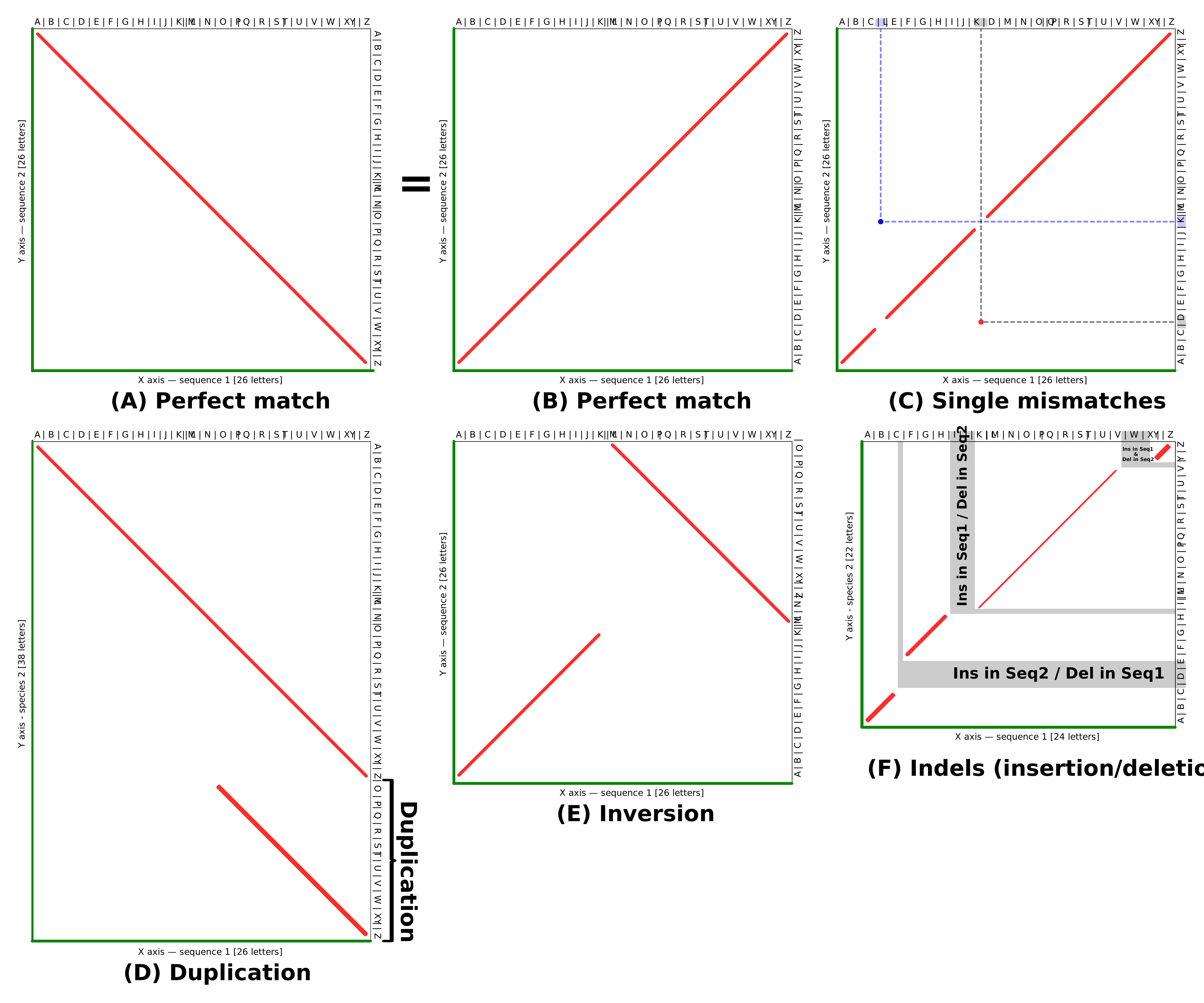
Figure 8. Dot plot interpretation.

Let’s remove the two shortest contigs (7 and 10) by editing contigs_to_keep.txt using nano :

Unix

cut -f1 assembly.fasta.fai > contigs_to_keep.txt

And running seqtk :

Unix

seqtk subseq assembly.fasta contigs_to_keep.txt > assembly_3_contigs.fasta

seqtk Toolkit for working with sequencing data
subseq Subcommand to extract sequences based on a list of identifiers
assembly.fasta The input FASTA file
contigs_to_keep.txt The text file containing a list of sequence IDs that we want to extract from the FASTA file
> Redirects the output of the command to a new file
assembly_3_contigs.fasta The output FASTA file containing only the specified sequences

[3] NextPolish

In order to improve the draft genome by identifying and correcting misassemblies and other inconsistencies, we will polish the assembly using highly accurate short and long (Illumina and HiFi) reads.

[A] Alignment

Here, we will align the HiFi reads on the draft assembly:

Unix

minimap2 -ax map-hifi -t 10 assembly_3_contigs.fasta HiFi_chr4_subset.fastq.gz | \
samtools sort -o hifi.map.sort.bam - && \
samtools index hifi.map.sort.bam

minimap2 Ultrafast sequence aligner for long reads
-ax Forces minimap2 to output in SAM format and defines parameters optimised for specific data types
map-hifi Preset optimized for PacBio HiFi reads
-t 10 Specifies 10 CPU threads for parallel alignment
assembly_3_contigs.fasta Reference genome
HiFi_chr4_subset.fastq.gz HiFi reads
| Indicates that output SAM-formatted alignments are streamed to the next command
samtools A set of tools for manipulating next-generation sequencing data
sort Sorts alignments by genomic coordinates
-o Indicates the output file
hifi.map.sort.bam The output file
- Takes input from stdin (the SAM data piped from minimap2)
&& Ensures that the next command (samtools index) is executed only if the previous command (samtools sort) succeeds
index Creates an index file for the sorted BAM file
hifi.map.sort.bam The output file (from the previous steps) and the input file for indexing

[B] K-mer dataset

Next, we will prepare two k-mer datasets by breaking Illumina reads into smaller pieces (k-mers). These k-mers can further improve the quality of our genome assembly by identifying and correcting errors such as sequencing mistakes or misassemblies:

Unix

yak count -o k21.yak -k 21 -b 37 <(zcat DNA_Illumina_chr4_subset_R*.fastq.gz) <(zcat DNA_Illumina_chr4_subset_R*.fastq.gz) &
yak count -o k31.yak -k 31 -b 37 <(zcat DNA_Illumina_chr4_subset_R*.fastq.gz) <(zcat DNA_Illumina_chr4_subset_R*.fastq.gz)

yak k-mer counting tool
count Subcommand performs k-mer counting on the input reads
-o Specifies the output file
k21.yak The output name
-k 21 Specifies the k-mer size
-b 37 Sets the number of bits used for hashing
<(zcat DNA_Illumina_chr4_subset_R*.fastq.gz) Decompresses and streams the contents of compressed FASTQ files directly into yak

[C] Polishing

Let’s then use both types of reads to polish the assembly:

Unix

nextPolish2 -r -t 10 hifi.map.sort.bam assembly_3_contigs.fasta k21.yak k31.yak > NP_genome.fa

nextPolish2 Corrects errors in the assembly
-r Specifies that the input alignment file
-t 10 Specifies the number of threads to use for parallel processing
hifi.map.sort.bam The input BAM file
assembly_3_contigs.fasta The reference sequence
k21.yak k31.yak k-mer count files
NP_genome.fa The final polished sequence

[D] Final notes

Additionally, we may want to reverse contig 6:

Unix

samtools faidx NP_genome.fa && \
cut -f1,2 NP_genome.fa.fai && \
(echo "contig_6" > contig_6.txt && \
seqtk subseq NP_genome.fa contig_6.txt | seqtk seq -r > reversed_contig_6.fa && \
grep '^>' NP_genome.fa | cut -d' ' -f1 | tr -d '>' | grep -v "contig_6" | \
seqtk subseq NP_genome.fa /dev/stdin > other_contigs.fa && \
cat other_contigs.fa reversed_contig_6.fa > Final_genome_with_Reference.fa)

echo "contig_6" > contig_6.txt Creates a text file containing only Contig 6
seqtk subseq NP_genome.fa contig_6.txt Extracts Contig 6 from the genome assembly
seqtk seq -r Reverses and complements the sequence (e.g., converting ACTG to CAGT)
grep '^>' NP_genome.fa Extracts all header lines starting with > from the FASTA file
cut -d' ' -f1 Removes any additional information after the header (e.g., >contig_1 info becomes >contig_1)
tr -d '>' Removes the > symbol from the headers, leaving only the sequence names
grep -v "contig_6" Excludes Contig 6 from the list of sequence names
seqtk subseq NP_genome.fa /dev/stdin Extracts sequences directly from the previous command
> other_contigs.fa Saves the extracted sequences to a new file
cat other_contigs.fa reversed_contig_6.fa Merges the reverse-complemented Contig 6 with the remaining contigs
Final_genome_with_Reference.fa The final combined concatenated FASTA file

And check the final assembly with D-Genies (Figure 9):

Figure 9. D-Genies: Reference vs the polished genome.

Assembly without a reference genome

If you have genome-wide chromatin interaction data (Hi-C), you can use it to scaffold contigs into chromosome-scale assemblies without requiring a reference genome.

To further explore this workflow, the following resources are recommended:
(1) The Genome Assembly Cookbook provides a detailed strategy for assembling chromosome-length genomes using Hi-C data.
(2) The Aiden Lab YouTube channel features instructional content on utilising Juicebox Assembly Tools for genome assembly visualisation and refinement.

IMPORTANT! Your directory structure must be correctly organised for Juicer to function. Follow the instructions closely.

Further to complete the assembly please follow the steps in this tutorial.

[IV] Genome annotation

Repeat identification and masking

Now, we need to identify and mask transposable elements prior to structural genome annotation.

[1] RepeatModeler

We will use RepeatModeler, a de novo Transposable Element family identification and modeling package.

First, we will create a formatted BLAST-compatible database from our genome sequence to facilitate repeat identification:

Unix

BuildDatabase -name A.thaliana.DB -engine rmblast Final_genome_with_Reference.fa

BuildDatabase Prepares a genome sequence into a database that can be used by RepeatMasker for repeat annotation
-name A.thaliana.DB Specifies the name of the database being created
-engine rmblast Specifies the search engine to use for building the database
Final_genome_with_Reference.fa The input FASTA file

And identify repetitive elements in the genome without relying on existing repeat libraries:

Unix

RepeatModeler -database A.thaliana.DB -engine rmblast -threads 10

RepeatModeler Identifies and classifies repetitive elements in genomic sequences
-database A.thaliana.DB Specifies the name of the database to analyse
-engine rmblast Specifies the search engine to use for building the database
-threads 10 Specifies the number of threads (CPU cores) to use for parallel processing

[2] RepeatMasker

Secondly, we will use RepeatMasker to mask the TEs identified by RepeatModeler:

Unix

RepeatMasker -pa 16 -xsmall -gff -lib consensi.fa.classified Final_genome_with_Reference.fa

RepeatMasker Identifies and masks repetitive elements
-pa 16 Specifies the number of parallel processes
-xsmall Softmasking (specifies that masked bases should be represented in lowercase instead of being replaced with N)
-gff Specifies output format (General Feature Format, GFF)
-lib consensi.fa.classified Specifies the custom repeat library to use for the analysis
Final_genome_with_Reference.fa The input FASTA file

Your results will be stored in a tabular file (see Final_genome_with_Reference.fa.tbl ):

==================================================
file name: Final_genome_with_Reference.fa
sequences:             3
total length:   19099067 bp  (19099067 bp excl N/X-runs)
GC level:         36.27 %
bases masked:    2565276 bp ( 13.43 %)
==================================================
               number of      length   percentage
               elements*    occupied  of sequence
--------------------------------------------------
Retroelements          950       908681 bp    4.76 %
   SINEs:                0            0 bp    0.00 %
   Penelope:             0            0 bp    0.00 %
   LINEs:              139        70941 bp    0.37 %
    CRE/SLACS            0            0 bp    0.00 %
     L2/CR1/Rex          0            0 bp    0.00 %
     R1/LOA/Jockey       0            0 bp    0.00 %
     R2/R4/NeSL          0            0 bp    0.00 %
     RTE/Bov-B           0            0 bp    0.00 %
     L1/CIN4           139        70941 bp    0.37 %
   LTR elements:       811       837740 bp    4.39 %
     BEL/Pao             0            0 bp    0.00 %
     Ty1/Copia          86        53177 bp    0.28 %
     Gypsy/DIRS1       725       784563 bp    4.11 %
       Retroviral        0            0 bp    0.00 %

DNA transposons        120        65243 bp    0.34 %
   hobo-Activator        0            0 bp    0.00 %
   Tc1-IS630-Pogo        0            0 bp    0.00 %
   En-Spm                0            0 bp    0.00 %
   MULE-MuDR            83        29184 bp    0.15 %
   PiggyBac              0            0 bp    0.00 %
   Tourist/Harbinger     0            0 bp    0.00 %
   Other (Mirage,        0            0 bp    0.00 %
    P-element, Transib)

Rolling-circles         26         5940 bp    0.03 %

Unclassified:         5043      1258310 bp    6.59 %

Total interspersed repeats:     2232234 bp   11.69 %


Small RNA:               0            0 bp    0.00 %

Satellites:              0            0 bp    0.00 %
Simple repeats:       5922       239827 bp    1.26 %
Low complexity:       1499        87275 bp    0.46 %
==================================================

* most repeats fragmented by insertions or deletions
  have been counted as one element

Please note that the current steps of repeat identification and masking are rather simplistic, and you may want to take a closer look at a more sophisticated approach, such as the one provided by Dr. Daren Card.

Structural annotation

In this step, we will use BRAKER3 to structurally annotate the assembled genome with RNA-Seq data and information from proteins of any evolutionary distance (see Figure 10).

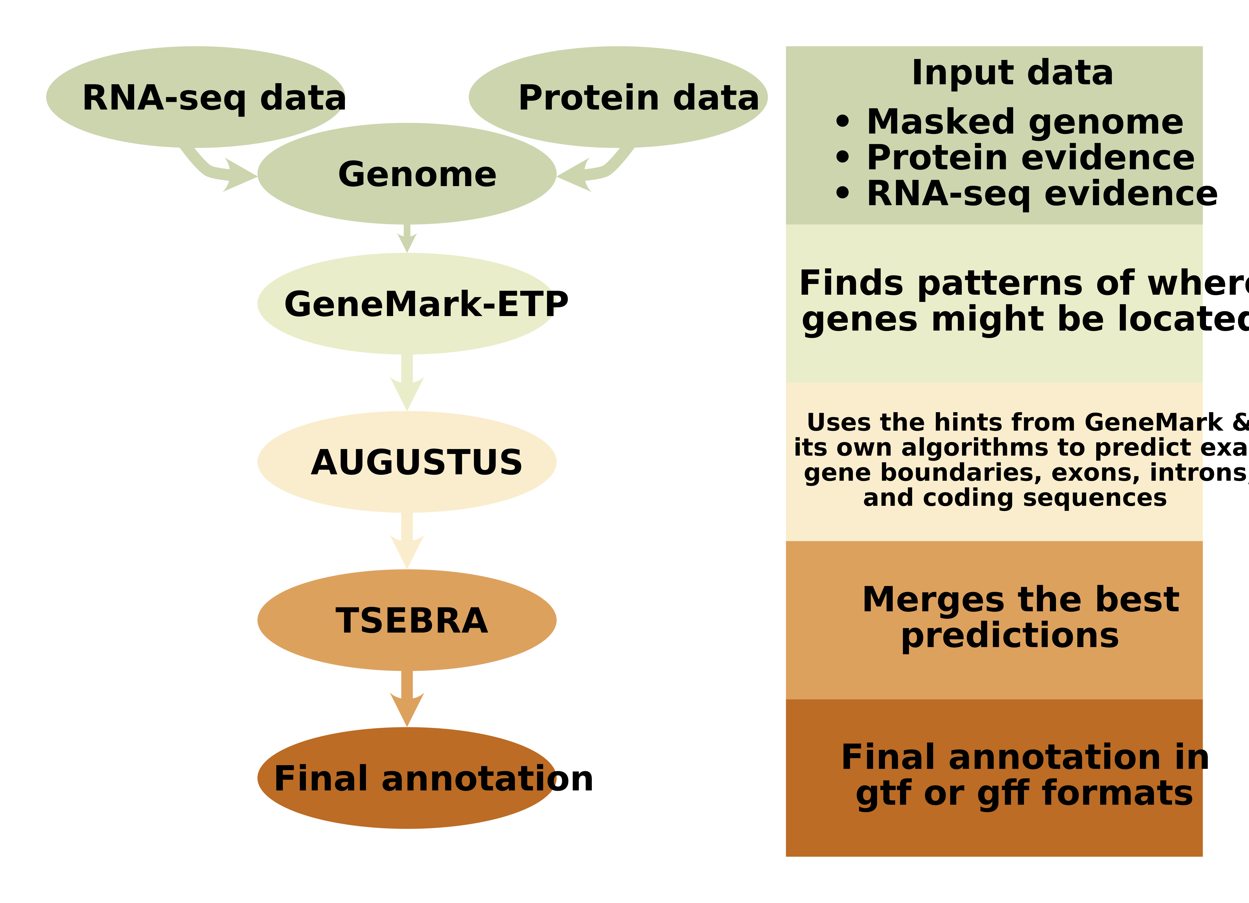
Figure 10. A simplified scheme of BRAKER3 pipeline with RNA and protein evidence.

First, we need to prepare the headers of the masked genome by retaining only the contig names:

Unix

sed -i 's/ start.*//' Final_genome_with_Reference.fa.masked

sed Editor used for text processing and manipulation
-i Edits the file in place (the changes are applied directly to the file)
's/ start.*//' Substitutes words matching start following by any characters with nothing
Final_genome_with_Reference.fa.masked The input file to be modified

Next, we need to download the latest protein evidence for green algae and land plants compatible with Braker3:

Unix

wget https://bioinf.uni-greifswald.de/bioinf/partitioned_odb12/Viridiplantae.fa.gz && \
gzip -d Viridiplantae.fa.gz

wget Utility to download files from the web
gzip -d Decompresses the downloaded file
Viridiplantae.fa.gz The final uncompressed file

Additionally, we need to index the masked genome:

Unix

hisat2-build Final_genome_with_Reference.fa.masked hisat2_masked_genome

hisat2-build Creates an index for the reference genome for fast and accurate alignment of sequencing reads
Final_genome_with_Reference.fa.masked The input genome file
hisat2_masked_genome Specifies the base name for the output index files

Then, we will map the RNA reads to the masked genome:

Unix

for sample in SRR3581706 SRR3581708 SRR3581693 SRR3581681 SRR3581356 SRR3581705 SRR3581703; do
    hisat2 -p 12 -x hisat2_masked_genome --rna-strandness F -U "${sample}_RNA_Illumina_chr4_subset.fastq" -S "${sample}.sam"
done

for sample in ...; do ... done A loop in Bash for a list of samples (SRR3581706, SRR3581708 ..)
hisat2 Aligns reads to a reference genome
-p 12 Specifies the number of threads (CPU cores) to use for parallel processing
-x hisat2_masked_genome Specifies the base name of the HISAT2 index files
--rna-strandness F Specifies the strandedness of the RNA-Seq data
-U Specifies the input FASTQ file containing single-end RNA-Seq reads
${sample} Will be replaced with the current sample ID in each iteration of the loop
-S "${sample}.sam" Specifies the output SAM file

Now, we will convert the .sam files into the .bam format:

Unix

for sample in SRR3581706 SRR3581708 SRR3581693 SRR3581681 SRR3581356 SRR3581705 SRR3581703; do
    samtools view --threads 16 -b -F 4 "${sample}.sam" > "${sample}.bam"
done

samtools view Reads the input SAM file
--threads 16 Specifies the number of threads (CPU cores) to use
-b Converts SAM to BAM
-F 4 Excludes unmapped reads

And subsequently sort these .bam files:

Unix

for sample in SRR3581706 SRR3581708 SRR3581693 SRR3581681 SRR3581356 SRR3581705 SRR3581703; do
  samtools sort -@ 4 -m 10G "${sample}.bam" -o "${sample}_sorted.bam"
done

samtools sort Sorts alignments in a BAM file by genomic coordinates
-@ 4 Specifies the number of threads (CPU cores) to use
-m 10G Specifies the maximum memory per thread for sorting

It is time to run Braker3:

Unix

nohup braker.pl --species=A.thaliana \
--genome=Final_genome_with_Reference.fa.masked \
--prot_seq=Viridiplantae.fa \
--bam=SRR3581706_sorted.bam,SRR3581708_sorted.bam,SRR3581693_sorted.bam,SRR3581681_sorted.bam,SRR3581356_sorted.bam,SRR3581705_sorted.bam,SRR3581703_sorted.bam, \
--threads=44 \
--gff3 &

nohup Runs the command in the background
braker.pl Runs BRAKER (a gene prediction pipeline)
--species=A.thaliana Specifies the species name for which gene predictions are being generated
--genome=Final_genome_with_Reference.fa.masked Specifies the input genome file
--prot_seq=Viridiplantae.fa Specifies a FASTA file containing protein sequences
--bam=SRR3581706_sorted.bam... Specifies a comma-separated list of sorted BAM files containing RNA-Seq alignments
--threads=44 Specifies the number of threads (CPU cores) to use
--gff3 Requests output in GFF3 format
& Runs the command in the background (allows you to continue using the terminal while BRAKER executes)

After, we need to collect some statistics on the resulted annotation:

Unix

agat_sp_statistics.pl --gff braker.gff3 -o AraTha_AGAT_stats

agat_sp_statistics.pl Computes various statistics about the genome annotation
--gff Specifies the input GFF3 file containing the genome annotation
braker.gff3 Runs BRAKER (a gene prediction pipeline)
-o AraTha_AGAT_stats Specifies the output file

Let’s check the result:

--------------------------------------------------------------------------------

Compute mrna with isoforms if any

Number of gene                               4252
Number of mrna                               4771
Number of cds                                4771
Number of exon                               24223
Number of intron                             19452
Number of start_codon                        4757
Number of stop_codon                         4769
Number of exon in cds                        24223
Number of intron in cds                      19452
Number of intron in exon                     19452
Number of intron in intron                   16034
Number gene overlapping                      38
Number of single exon gene                   1240
Number of single exon mrna                   1353
mean mrnas per gene                          1.1
mean cdss per mrna                           1.0
mean exons per mrna                          5.1
mean introns per mrna                        4.1
mean start_codons per mrna                   1.0
mean stop_codons per mrna                    1.0
mean exons per cds                           5.1
mean introns in cdss per mrna                4.1
mean introns in exons per mrna               4.1
mean introns in introns per mrna             3.4
Total gene length                            7678231
Total mrna length                            8842281
Total cds length                             5807925
Total exon length                            5807925
Total intron length                          3034356
Total start_codon length                     14267
Total stop_codon length                      14307
Total intron length per cds                  3034356
Total intron length per exon                 3034356
Total intron length per intron               2683871
....................................................
--------------------------------------------------------------------------------

For the downstream quality check with BUSCO, we will retain only the longest isoforms:

Unix

agat_sp_keep_longest_isoform.pl \
   -gff braker.gff3 \
   -o longest_isoform_only.gff3

agat_sp_keep_longest_isoform.pl Identifies and retains only the longest transcripts for each gene
-gff braker.gff3 Specifies the input GFF3 file
-o longest_isoform_only.gff3 Specifies the output file name

And extract these protein sequences from the masked genome:

Unix

agat_sp_extract_sequences.pl \
   --gff longest_isoform_only.gff3 \
   -f Final_genome_with_Reference.fa.masked \
   -p \
   -o longest_isoform_only.fa

agat_sp_extract_sequences.pl Extract sequences based on annotations in a GFF3 file
--gff longest_isoform_only.gff3 Specifies the input
-f Final_genome_with_Reference.fa.masked Specifies the input genome
-p Requests extraction of protein sequences instead of nucleotide sequences
-o longest_isoform_only.fa Specifies the output file

[V] Quality assessment

BUSCO

To assess genome assembly and annotation completeness, we will use Benchmarking Universal Single-Copy Orthologs (BUSCO). Specifically, we will compare (1) the original genome assembly versus the one assembled here and (2) the predicted number of BUSCOs in the assembled genome versus the number of detected proteins with BRAKER.

Let’s first check the reference Chromosome 4:

Unix

busco \
   -m genome \
   -i Arabidopsis_GWHBDNP00000000_chr4.fasta \
   -o Embryophyta_1614_Ref_Genome \
   -l embryophyta_odb10 \
   --offline \
   --download_path busco_downloads \
   -c 22

busco Evaluates the completeness of genome assemblies,
-m genome Specifies the mode of operation
-i Arabidopsis_GWHBDNP00000000_chr4.fasta The input file
-o Embryophyta_1614_Ref_Genome Specifies the output file
-l embryophyta_odb10 Specifies the lineage dataset to use
--offline Enables offline mode (BUSCO uses pre-downloaded datasets)
--download_path busco_downloads Specifies the directory where BUSCO datasets are stored
-c 22 Specifies the number of CPU threads to use

And our de novo assembled Chromosome 4:

Unix

busco \
   -m genome \
   -i Final_genome_with_Reference.fa.masked \
   -o Embryophyta_1614_Workshop_Genome \
   -l embryophyta_odb10 \
   --offline \
   --download_path busco_downloads \
   -c 22

Lastly, we will assess BUSCOs with the pre-computed protein sequences:

Unix

busco \
   -m protein \
   -i longest_isoform_only.fa \
   -o Embryophyta_Workshop_Protein_1614 \
   -l embryophyta_odb10 \
   --offline \
   --download_path busco_downloads \
   -c 44

Please note that you can also run BUSCO online using the web-based platform Galaxy.

Time to check the results (Figure 11):

Figure 11. BUSCO assessment results across the three datasets (Chromosome 4).

IMPORTANT! BUSCO has several algorithms that can potentially lead to different assessments of genome completeness [genome mode]. (1) Miniprot yields slightly higher completeness scores compared to Augustus and MetaEuk, making it a good choice for large genomes or when runtime is critical; (2) MetaEuk is very fast, especially for smaller genomes like fungi, though it may be slower than Miniprot for larger genomes; (3) Augustus is slower than both Miniprot and MetaEuk but is recommended when precise gene predictions are needed and you have time to optimise parameters. Additionally, the protein mode is standardised, there are no alternative tools (e.g., Miniprot vs. MetaEuk).

QUAST

Next, to gather additional statistics on our assembly, we will use the QUality ASsessment Tool (QUAST):

Unix

quast.py \
Final_genome_with_Reference.fa.masked \
-r Arabidopsis_GWHBDNP00000000_chr4.fasta \
--min-alignment 20000 \
--extensive-mis-size 500000 \
--min-identity 90 \
--threads 44

quast.py Assesses the quality of genome assemblies
Final_genome_with_Reference.fa.masked Specifies the input genome
-r Arabidopsis_GWHBDNP00000000_chr4.fasta Specifies the reference genome
--min-alignment 20000 Specifies the min alignment length required for alignments between assembly and reference
--extensive-mis-size 500000 Specifies the threshold for classifying large misassemblies
--min-identity 90 Specifies the min sequence identity required for alignments between assembly and reference
--threads 44 Specifies the number of CPU threads to use

Let’s see the results (Figure 12):

Figure 12. Quality assessment statistics generated by QUAST.

Dot plot

Here, we can also use a dot plot (Figure 9 = Figure 13) to provide an intuitive, global view of how an assembled genome aligns to a reference (if available). Tools like QUAST or BUSCO offer quantitative metrics (e.g., N50, misassemblies, completeness), but dot plots add qualitative context. For instance, a dot plot can confirm that a genome is correctly ordered and oriented, even if QUAST flags minor misassemblies.

Figure 13. Dot plot produced by D-Genies: Reference versus the genome assembled in this tutorial.

Synteny

Another way to verify if our assembly is correctly ordered and oriented is by comparing the gene order (Figure 14) in the newly assembled genome with the reference. This comparison helps evaluate large-scale structural accuracy. Additionally, syntenic plots are commonly used in comparative genomics to highlight similarities and differences between genomes of interest.

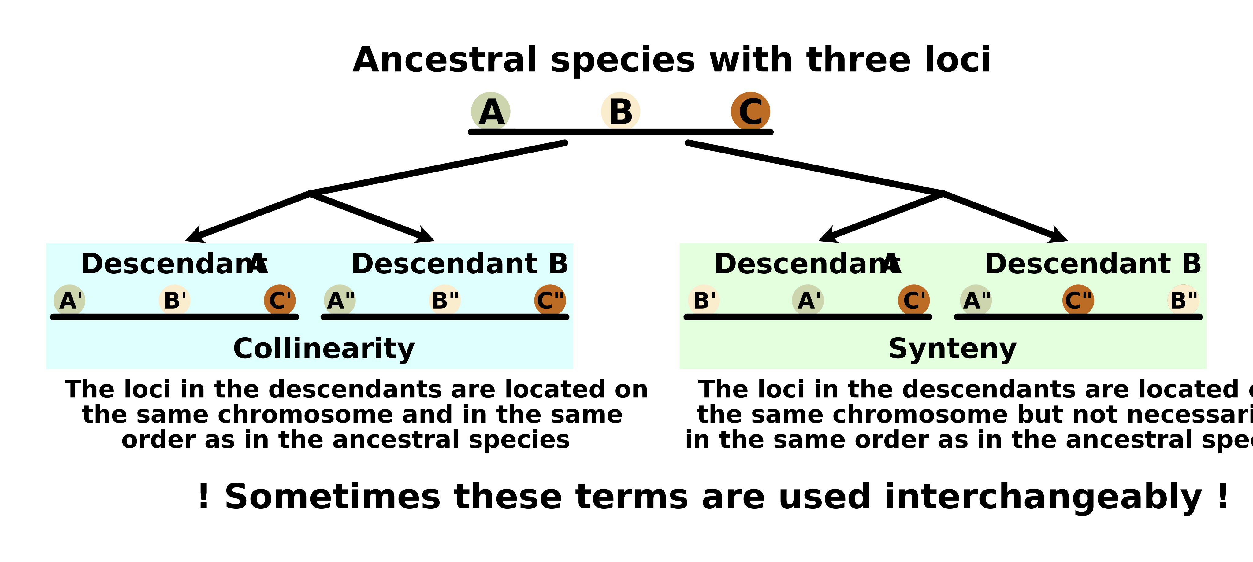
Figure 14. A visual explanation of the terms collinearity and synteny.

Here, we will compare the whole genomes of Arabidopsis thaliana and Arabidopsis arenosa. First, we will download their nucleotide sequences and annotated genomes:

Unix

wget https://ftp.ncbi.nlm.nih.gov/genomes/all/GCA/905/216/605/GCA_905216605.1_AARE701a/GCA_905216605.1_AARE701a_genomic.gff.gz && pigz -d GCA_905216605.1_AARE701a_genomic.gff.gz && \
wget https://ftp.ncbi.nlm.nih.gov/genomes/all/GCA/905/216/605/GCA_905216605.1_AARE701a/GCA_905216605.1_AARE701a_genomic.fna.gz && pigz -d GCA_905216605.1_AARE701a_genomic.fna.gz && \
wget https://ftp.ncbi.nlm.nih.gov/genomes/all/GCF/000/001/735/GCF_000001735.4_TAIR10.1/GCF_000001735.4_TAIR10.1_genomic.gff.gz && pigz -d GCF_000001735.4_TAIR10.1_genomic.gff.gz && \
wget https://ftp.ncbi.nlm.nih.gov/genomes/all/GCF/000/001/735/GCF_000001735.4_TAIR10.1/GCF_000001735.4_TAIR10.1_genomic.fna.gz && pigz -d GCF_000001735.4_TAIR10.1_genomic.fna.gz

We will keep only the longest isoforms:

Unix

agat_sp_keep_longest_isoform.pl -gff GCA_905216605.1_AARE701a_genomic.gff \
-o AraAre_longest_isoform_only.gff3 \
&& \
agat_sp_keep_longest_isoform.pl -gff GCF_000001735.4_TAIR10.1_genomic.gff \
-o AraTha_longest_isoform_only.gff3

IMPORTANT! I had to remove some entries from AraTha_longest_isoform_only.gff3 that were causing errors in the next steps:

Unix

grep -v -E '(ID|Parent)=(agat-gene-351|rna-DA397_mgp37)(;|$)' \
AraTha_longest_isoform_only.gff3 > AraTha_longest_isoform_only_corrected.gff3 \
&& \
awk 'NR==FNR { len[$1]=$2; next } $1 in len && ($4 > len[$1] || $5 > len[$1]) { print "Invalid:" $0 }' \
GCF_000001735.4_TAIR10.1_genomic.fna.fai AraTha_longest_isoform_only_corrected.gff3

We also need to create index files to enable efficient access to specific regions of the genomes in subsequent steps:

Unix

samtools faidx GCF_000001735.4_TAIR10.1_genomic.fna \
&& \
samtools faidx GCA_905216605.1_AARE701a_genomic.fna

Next, we need to get the transcript sequences:

Unix

gffread -g GCA_905216605.1_AARE701a_genomic.fna \
-w AraAre_transcripts.fa AraAre_longest_isoform_only.gff3 \
&& \   
gffread -g GCF_000001735.4_TAIR10.1_genomic.fna \
-w AraTha_transcripts.fa AraTha_longest_isoform_only_corrected.gff3

gffread Calls the tool for processing GFF/GTF files
-g GCA_905216605.1_AARE701a_genomic.fna Specifies the input genome
-w AraAre_transcripts.fa AraAre_longest_isoform_only.gff3 Requests extraction of transcript sequences in FASTA format

Here, we will convert GFF3 into a simpler format used for genomic annotations (Browser Extensible Data or BED):

Unix

python -m jcvi.formats.gff bed --type=mRNA --key=ID AraAre_longest_isoform_only.gff3 \
-o AraAre.bed \
&& \
python -m jcvi.formats.gff bed --type=mRNA --key=ID AraTha_longest_isoform_only_corrected.gff3 -o AraTha.bed

python Invokes the Python interpreter
-m Specifies a jcvi module
jcvi.formats.gff bed Converts a GFF3 file into BED format
--type=mRNA Specifies the feature type to extract from the GFF3 file (mRNA here)
---key=ID Specifies the attribute to use as the name for each BED entry
AraAre_longest_isoform_only.gff3 The input file

Subsequently, we need to retrieve the coding sequences (CDS) from the transcripts:

Unix

python -m jcvi.formats.fasta format AraTha_transcripts.fa AraTha.cds \
&& \
python -m jcvi.formats.fasta format AraAre_transcripts.fa AraAre.cds

jcvi.formats.fasta format Processes and reformates a FASTA file by extracting CDS
AraTha_transcripts.fa Specifies the input file
AraTha.cds Specifies the output file

Next, we will perform a pairwise synteny search:

Unix

python -m jcvi.compara.catalog ortholog AraTha AraAre --no_strip_names

jcvi.compara.catalog ortholog Identifies orthologous gene pairs between two species based on their genome annotations
AraTha AraAre The pair of species being compared
--no_strip_names Preserves the original names in the output

Here, we need to perform a filtering step on synteny anchors to refine the results of the synteny analysis:

Unix

python -m jcvi.compara.synteny screen --simple --minspan=30 AraTha.AraAre.anchors AraTha.AraAre.anchors.anchors.new

jcvi.compara.synteny screen Filters and refines orthologous gene pairs based on user-defined criteria
--simple Simplifies the filtering process by focusing only on basic criteria
--minspan=30 Specifies the minimum number of anchor pairs required for a synteny block to be retained
AraTha.AraAre.anchors The input file containing the initial set of orthologous gene pairs between the species
AraTha.AraAre.anchors.anchors.new Preserves the original names in the output

Additionally, we need to create two files. On is seqids containing chromosome names of our two genomes:

LR999451.1,LR999452.1,LR999453.1,LR999454.1,LR999455.1,LR999456.1,LR999457.1,LR999458.1
NC_003070.9,NC_003071.7,NC_003074.8,NC_003075.7,NC_003076.8

The second one is layout, describing how we want our data to be rendered:

# y, xstart, xend, rotation, color, label, va,  bed
 .6,     .1,    .8,       0,      , AraAre, center, AraAre.bed
 .4,     .1,    .8,       0,      , AraTha, center, AraTha.bed
# edges
e, 0, 1, AraTha.AraAre.anchors.anchors.simple

Finally, we will plot the results (Figure 15):

Unix

python -m jcvi.graphics.karyotype seqids layout --chrstyle=roundrect --basepair

jcvi.graphics.karyotype Invokes the karyotype plotting module from the jcvi library
seqids A file listing the chromosome/contig identifiers (e.g., chr1, chr2) to include in the plot
layout A configuration file specifying the arrangement of chromosomes in the plot (e.g., rows, spacing, colors)
--chrstyle=roundrect Draws chromosomes as rounded rectangles instead of default rectangles
--basepair Adds a scale bar to the plot, labeled in base pairs

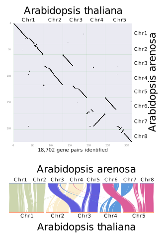
Figure 15. Dot plot (top) and syntenic blocks (bottom) identified by jcvi.

Additionally, please consider using this tutorial for more detailed comparative analysis and visualisation steps.

You may also check my previous tutorial on additional tools you can use to assess the quality of your newly-assembled genomes.

[VI] Software reference

This section lists the software versions used in the Conda environment to ensure reproducibility and consistency:

agat=1.1.0 
braker3=3.0.8
busco=5.8.2
cutadapt=5.0
dgenies=1.5.0
fastqc=0.12.1 
flye=2.9.5
gffread=0.12.7
hisat2=2.2.1 
jcvi=1.4.16
juicer_tools=2.20.00
minimap2=2.28  
nanoplot=1.44.0 
necat=0.0.1_update20200803
nextpolish2=0.2.1 
parallel=20240122
pigz=2.8
porechop=0.2.4
quast=5.3.0
repeatmasker=4.1.5 
repeatmodeler=2.0.4 
samtools=1.21  
seqtk=1.4 
sra-tools=2.9.6
trim-galore=0.6.10
wget=1.21.4

[VII] Cite

Baiakhmetov E. (2025). Quality check and genome assembly using Illumina, ONT, HiFi, and Hi-C data [Tutorial]. GitHub. https://niwdoog.github.io/Genome_Assembly_XTBG_2025

GWHBDNP00000001	Chromosome 1	Complete=F	Circular=F	OriSeqID=chr1	Len=32659241
GWHBDNP00000002	Chromosome 2	Complete=F	Circular=F	OriSeqID=chr2	Len=22712559
GWHBDNP00000003	Chromosome 3	Complete=F	Circular=F	OriSeqID=chr3	Len=26161332
GWHBDNP00000004	Chromosome 4	Complete=F	Circular=F	OriSeqID=chr4	Len=22250686
GWHBDNP00000005	Chromosome 5	Complete=F	Circular=F	OriSeqID=chr5	Len=30093473

contig_10	7816
contig_3	3244749
contig_5	959609
contig_6	14850431
contig_7	12283

Quality check and genome assembly using Illumina, ONT, HiFi, and Hi-C data

Created by Evgenii Baiakhmetov

[I] Preface

In a nutshell

Learning outcomes

Keywords

[II] Conda & sequencing data

Conda, software, and packages

Downloading raw sequence data

Subsampling workflow

[1] Dataset

[2] Chromosome subsetting

[3] Trimming and alignment

Illumina DNA data

Illumina RNA data

Illumina Hi-C data

PacBio HiFi data

ONT data

[4] Sabsampling for the QC chapter

Illumina DNA data

PacBio HiFi data

ONT data

[III] Genome assembly

Recap

Quality check

Short-Read Sequencing

Long-Read Sequencing

[1] PacBio HiFi reads

[2] ONT reads

Assembly with a reference genome

[1] Flye

[2] D-Genies

[3] NextPolish

[A] Alignment

[B] K-mer dataset

[C] Polishing

[D] Final notes

Assembly without a reference genome

[IV] Genome annotation

Repeat identification and masking

[1] RepeatModeler

[2] RepeatMasker

Structural annotation

[V] Quality assessment

BUSCO

QUAST

Dot plot

Synteny

More

[VI] Software reference

[VII] Cite